Picture this: You are playing Snakes and Ladder and need the dice to roll the same way every time. Sounds a bit like cheating, right? In R, you can have this superpower, introducing the set.seed() function.
The set.seed() function sets the seed of R’s random number generator.
The set.seed() function replicates the exact reproducible random numbers, which means it will help create the same random numbers every time you call the random function like rnorm().
But why does anyone want to predict randomness? In data science and statistics, reproducing your results is like having a golden ticket. It’s all about credibility and being able to say, “Look, I’m not making this up! You can get the same results too!”
Why should you use it?
By using the set.seed() function, you ensure that the code returns the same sequence of random numbers every time.
When you debug the application, if you fix the seed of the random number, it will be easy to generate the same random number and debug the application, leading to arriving at the problem. If your seed changes, then the problem in your code will keep changing.
The set.seed() function will work as a “rewind” button, where you will rerun the scenario multiple times and expect the same result.
This method is beneficial when comparing different random number generation algorithms, where each algorithm gets the same random number, making a fair comparison. If you share your code with others, including the seed value you used, they can replicate your results.
Basic syntax and parameters
set.seed(value)
| Name | Description |
| value | It is the single value that sets the R’s random number generator. It is an integer and determines the sequence of random numbers. |
Example 1: Basic usage
Before using the set.seed() function, let’s generate a random number:
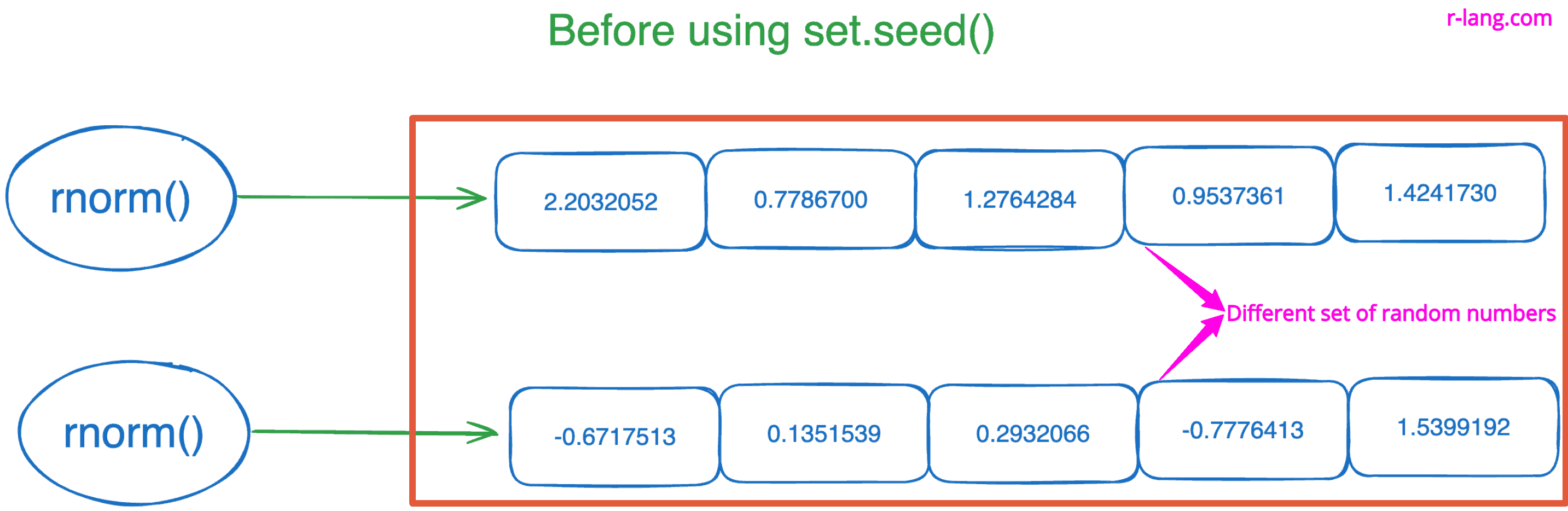
The above figure shows that both results are different, which means that every time you run the code, you will get five different random numbers.
x <- rnorm(5)
print(x)

cat("Let's generate random number again", "\n")

y <- rnorm(5)
print(y)
Output
[1] 2.2032052 0.7786700 1.2764284 0.9537361 1.4241730

Let's generate random number again

[1] -0.6717513 0.1351539 0.2932066 -0.7776413 1.5399192
We used the rnorm() function to generate the random numbers.
After using the set.seed() function:
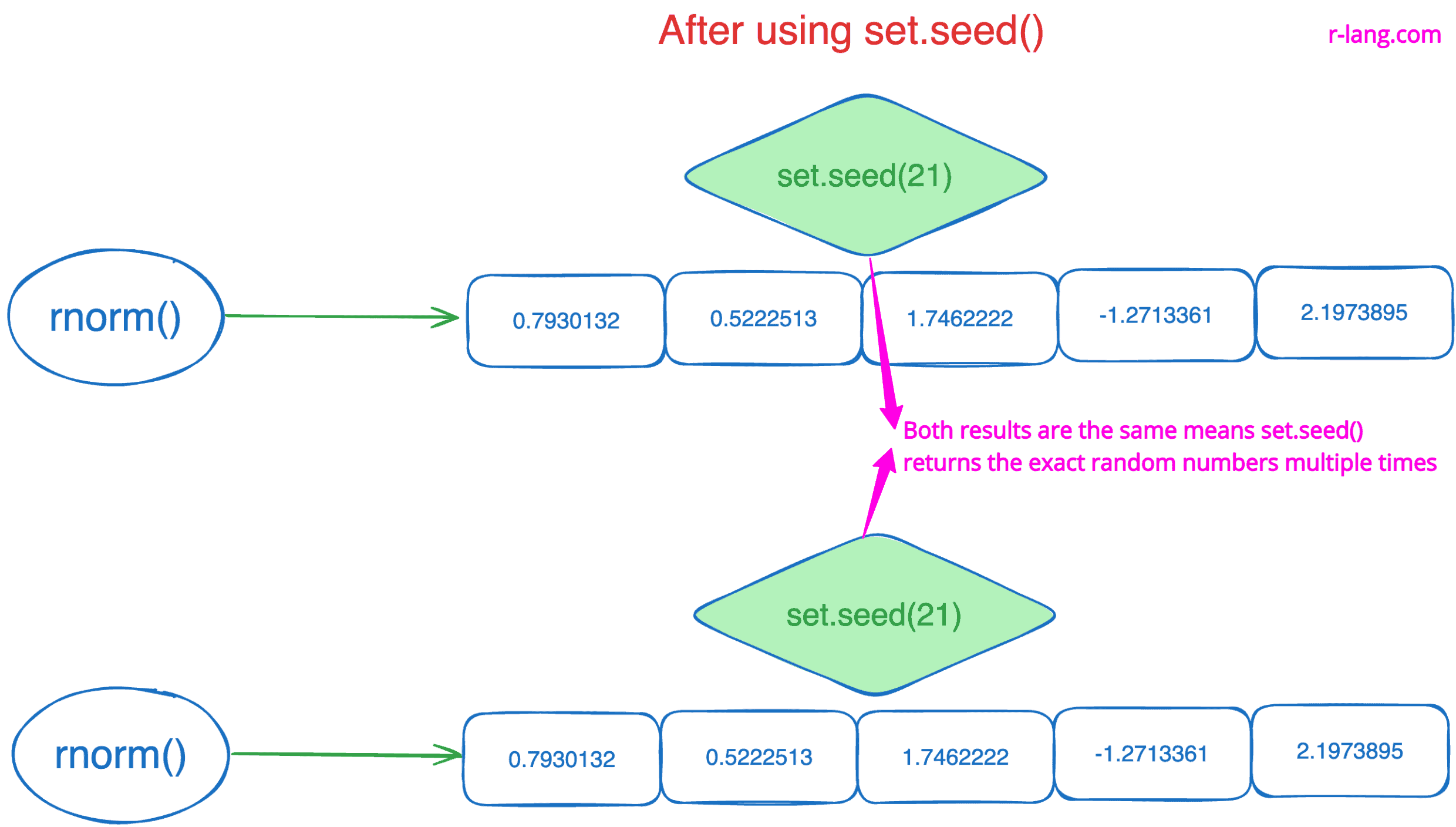
The above figure shows that when you set the seed to 21, the code reproduces the same set of random numbers every time it is run.
Here, the main ingredient is 21. You can set whichever you want, and it will generate the random number based on that. However, when you run the program multiple times, it will return the same output.
set.seed(21)

x <- rnorm(5)
print(x)

cat("Let's generate random number again after setting the seed", "\n")

set.seed(21)

y <- rnorm(5)
print(y)
Output
[1] 0.7930132 0.5222513 1.7462222 -1.2713361 2.1973895

Let's generate random number again after setting the seed

[1] 0.7930132 0.5222513 1.7462222 -1.2713361 2.1973895
Voila! We get the exact output every time we run the code because we fixed the seed, and now R will generate the same number in any machine anywhere in the world.
Example 2: Basic random data visualization
# Setting the seed for reproducibility
set.seed(123)

# Generating random data
data <- rnorm(100, mean = 50, sd = 10)

# Basic plot
hist(data,
  main = "Histogram of Normally Distributed Data",
  xlab = "Values",
  col = "blue",
  border = "black")
Output
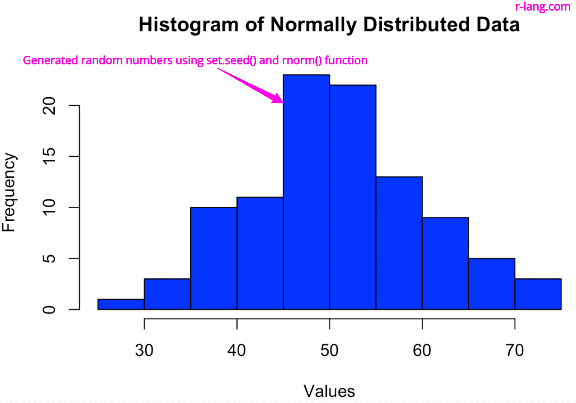
If you run the above code in your system, you will also get the same chart as me. Since we fixed the seed, it will generate the same random number and hence the same above chart of normally distributed data.
Example 3: Multiple datasets comparison
# Setting seed
set.seed(123)
# Generating two sets of random data
data1 <- rnorm(100, mean = 50, sd = 10)
data2 <- rnorm(100, mean = 55, sd = 15)
data3 <- rnorm(100, mean = 45, sd = 20)
# Plotting both datasets
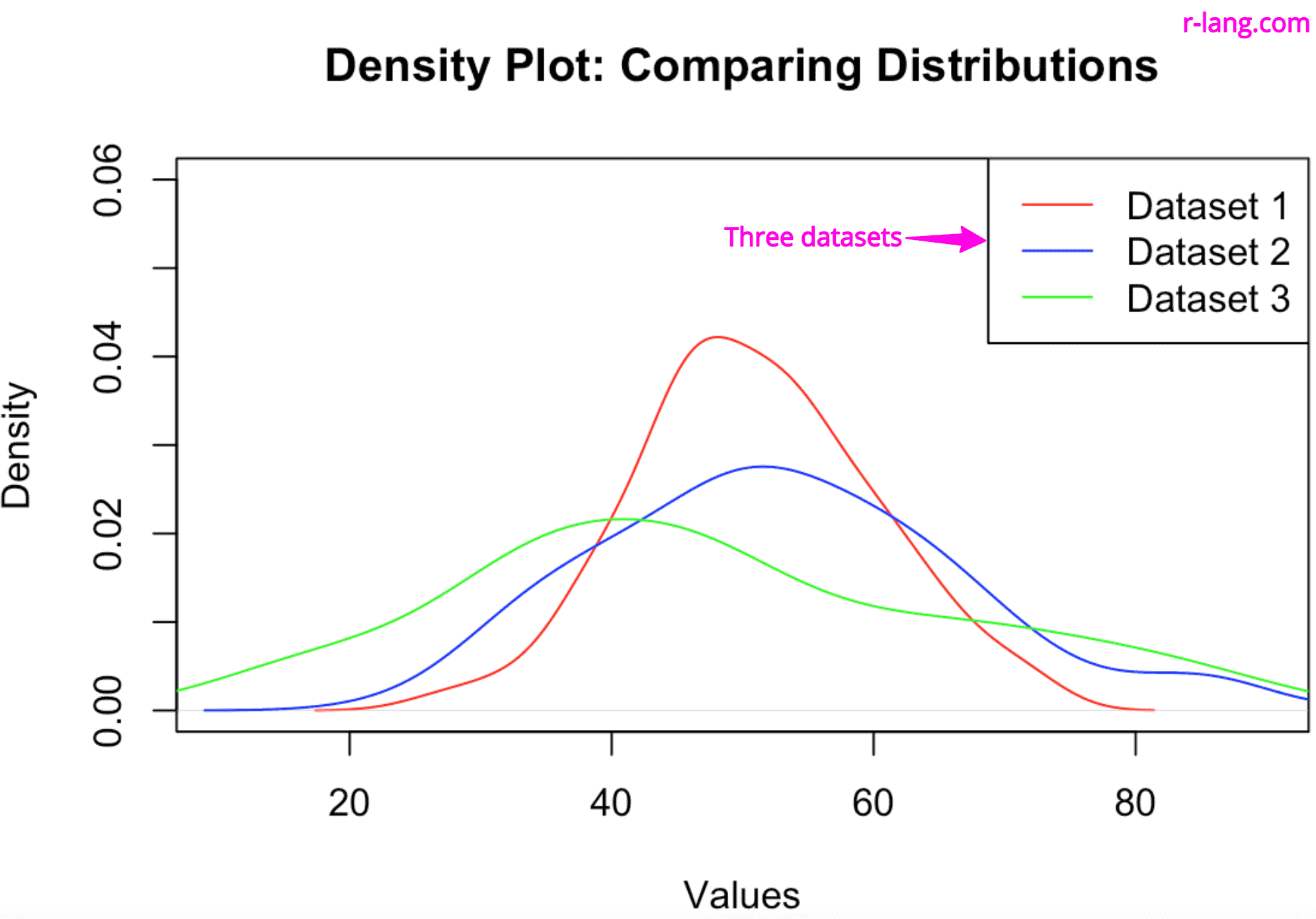
plot(density(data1),
col = "red",
main = "Density Plot: Comparing Distributions",
xlim = c(10, 90),
ylim = c(0, 0.06),
xlab = "Values",
ylab = "Density")
lines(density(data2), col = "blue")
lines(density(data3), col = "green")
legend("topright",
legend = c("Dataset 1", "Dataset 2", "Dataset 3"),
col = c("red", "blue", "green"),
lty = 1)
Output
That’s all!

Krunal Lathiya is a seasoned Computer Science expert with over eight years in the tech industry. He boasts deep knowledge in Data Science and Machine Learning. Versed in Python, JavaScript, PHP, R, and Golang. Skilled in frameworks like Angular and React and platforms such as Node.js. His expertise spans both front-end and back-end development. His proficiency in the Python language stands as a testament to his versatility and commitment to the craft.