
The dnorm() function in R calculates the value of the probability density function (pdf) of the normal distribution of a given value or vector of values.
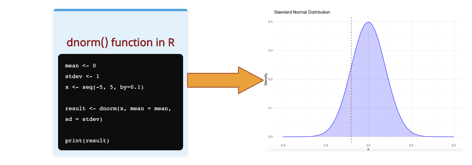
It determines the probability density of a continuous random variable following a normal distribution, characterized by a mean (μ) and standard deviation (σ).
How do you define the normal distribution? Well, think like a mountain that is tallest in the middle and slopes down on both sides.
Now, if someone asks, ‘How tall is the mountain at this specific point?’ Well, the answer is the dnorm() function. It indicates the height of the hill at a specific location.
The output of this function is non-negative but not a probability (densities can exceed 1, unlike probabilities).
Syntax
dnorm(x, mean = 0, sd = 1, log = FALSE)
Parameters
| Argument | Description |
| x | It represents a vector of quantiles whose density you want to evaluate. |
| mean | It is a mean of normal distribution. By default, it is 0. |
| sd | It is the standard deviation of a normal distribution. By default, its value is 1, and it must be positive. |
| log | It is a logical argument that is FALSE by default. If TRUE, it returns the logarithm of the density. |
Standard normal distribution
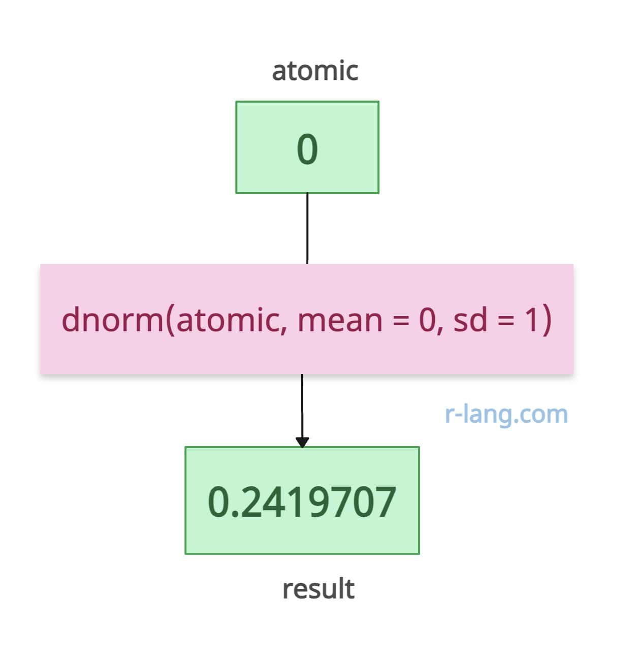
atomic <- -1

result <- dnorm(atomic, mean = 0, sd = 1)

print(result)

# Output: [1] 0.2419707
Vectorized input
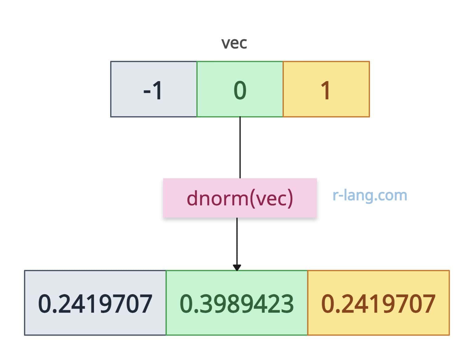
What if an input is a vector? Well, it is a vectorized function, which means it will operate element-wise on vectors, making it efficient for multiple inputs.
vec <- c(-1, 0, 1)

dnorm(vec)

# Output: [1] 0.2419707 0.3989423 0.2419707
Custom mean and standard deviation
Let’s not use the default values of mean and standard deviation; instead, we will pass custom values and evaluate the density for a normal distribution.
dnorm(21, mean = 21, sd = 11)
# Output: [1] 0.03626748

# Vector input
vec <- c(8, 11, 14)

dnorm(vec, mean = 10, sd = 2)
# Output: [1] 0.12098536 0.17603266 0.02699548
Smaller SD values create a sharper peak. Wider SD values create a blunt hill.
dnorm(0)
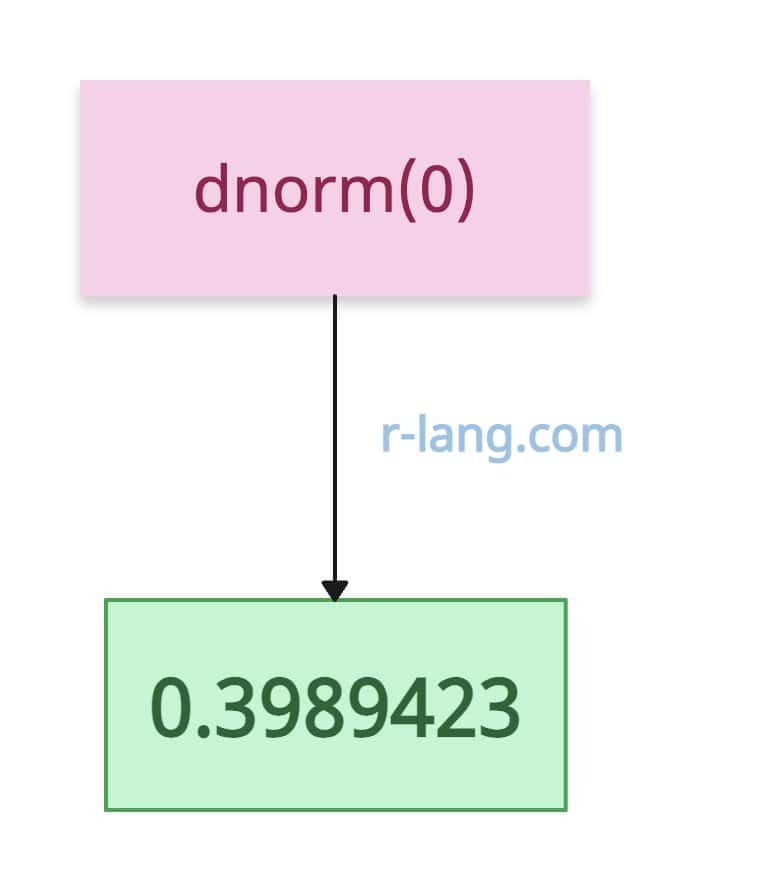
dt <- dnorm(0)

dt

# Output: [1] 0.3989423
Log-density
For computation stability, we can obtain the log of the density.
dnorm(0, log = TRUE)
# Output: [1] -0.9189385 (log of 0.3989423)

dnorm(c(-1, 0, 1), log = TRUE)
# Output: [1] -1.4189385 -0.9189385 -1.4189385
The log = TRUE argument is extremely helpful for numerical stability when density values are minimal.
Plotting
To plot a probability distribution function, we can use the plot() method.
seq(-4, 4, by = 0.05)

result <- dnorm(seq(-4, 4, by = 0.05))

plot(result)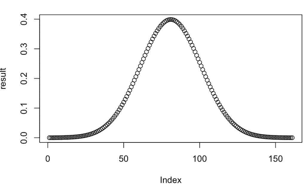
Using ggplot2
library(ggplot2)

# Generate x values
x_values <- seq(-5, 5, by = 0.025)

# Compute y values using the dnorm function
y_values <- dnorm(x_values, mean = 0, sd = 1)

# Point of interest
poi_x <- 0
poi_y <- dnorm(poi_x, mean = 0, sd = 1)

# Plotting
df <- data.frame(x = x_values, y = y_values)
ggplot(df, aes(x, y)) +
  geom_line(color = "blue") +
  geom_point(aes(x = poi_x, y = poi_y), color = "red", size = 4) +
  labs(
    title = "Density of Standard Normal Distribution at x=0",
    x = "x", y = "Density"
  ) +
  theme_minimal() +
  theme(legend.position = "none")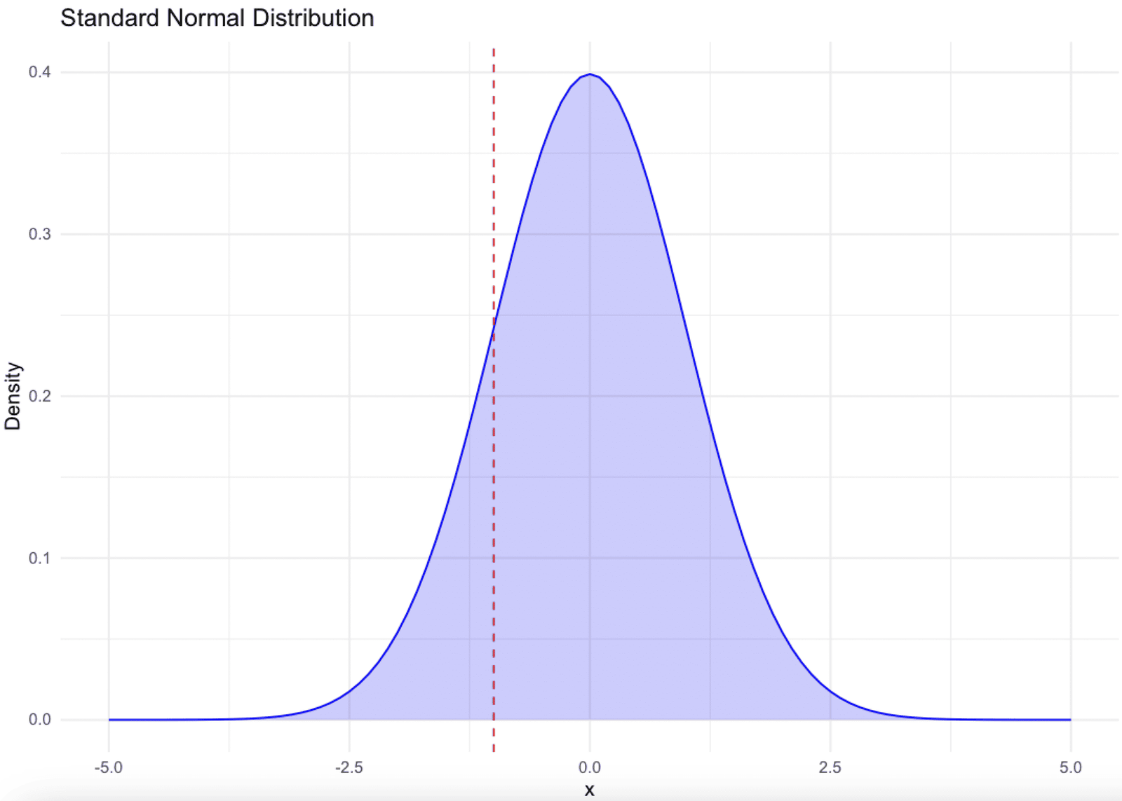
Calculating probability density for a range of values
You can calculate the probability density for a range of values using this function in combination with the sapply() function.
x <- c(-3, -2, -1, 0, 1, 2, 3)
mean <- 0
sd <- 1
log <- FALSE

sapply(x, dnorm, mean=mean, sd=sd, log=log)
Output
[1] 0.004431848 0.053990967 0.241970725 0.398942280 0.241970725 0.053990967
[7] 0.004431848
Invalid Standard Deviation
What if your input standard deviation is invalid. What do I mean by that is what if it is negative or 0 because it can’t be negative. If that is the case, it will throw the error.
Well, sd = 0 means the curve of the hill is infinity and there is no spread. That means, all the probability is squished into a single point and the output will inf, which won’t be the case in real-time calculations.
dnorm(0, mean = 0, sd = 0)

# Output: [1] Inf
Now, let’s talk about the second usecase, which is if SD is negative. That won’t be possible to because if we are talking about a hill, then its spread is a distance and it cannot be negative because the distance is always positive.
If you pass negative SD, it will return NaN.
dnorm(0, mean = 0, sd = -1)

# Output: [1] NaN
That’s all!

Krunal Lathiya is a seasoned Computer Science expert with over eight years in the tech industry. He boasts deep knowledge in Data Science and Machine Learning. Versed in Python, JavaScript, PHP, R, and Golang. Skilled in frameworks like Angular and React and platforms such as Node.js. His expertise spans both front-end and back-end development. His proficiency in the Python language stands as a testament to his versatility and commitment to the craft.