To calculate the sample variance (measurement of spreading) in R, you should use the built-in var() function. It calculates the sample variance (using n−1 for unbiased estimation, where n is the sample size). By default, it does not calculate the population variance.
Variance measures how spread out a set of numbers is around the mean (average). If the variance is a small number, it is close to the mean value. If the variance is a high number, it is very far from the mean value, which means it is spread out.
If variance becomes 0, all the data points become identical. Variance cannot have a negative value.
Syntax
var(x, y = NULL, na.rm = FALSE, use)Parameters
| Name | Value |
| x | It is a numeric vector, matrix, or data frame |
| y | It is the second vector or matrix for covariance calculation. |
| na.rm | By default, it is FALSE, but if TRUE, it removes missing values (NA). |
| use | It specifies how to handle missing values in matrices or data frames. |
Return value
It returns the variance of the input vector. If your input is a data frame, it returns a covariance matrix if y is provided or if the input has more than one column.
Variance of a numeric vector

vec <- c(60, 55, 50, 65, 59)

var(vec)

# Output: [1] 31.7
Handling NA values
If your data contains NA values, it will return NA as an output.
vec <- c(60, 55, 50, NA, 59)

var(vec)

# Output: [1] NA
To exclude them from the calculation, pass the na.rm = TRUE to the function.
vec <- c(60, 55, 50, NA, 59)

var(vec, na.rm = TRUE)

# Output: [1] 20.66667
Using a real-life dataset
Step 1: Install the libraries
We need “tidyverse” and “ggplot2” libraries to continue this small project.
install.packages("tidyverse")

install.packages("ggplot2")
Step 2: Import and Load the Dataset
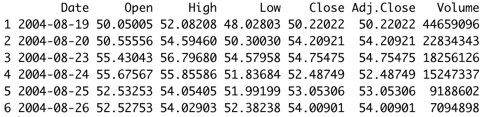
We will use Kaggle’s Google Stock Data.
library(tidyverse)
library(ggplot2)

google_data <- read_csv("./DataSets/GOOGL.csv")

head(google_data)
Output
Step 3: Calculation of Variance
# Calculate variance for each numerical column
variance_data <- sapply(select(google_data, -Date), var)

variance_data
Output

Step 4: Visualize the Variance
To visualize the variance data, we can create a barplot where the x-axis represents the features (columns) of the dataset and the y-axis represents their respective variance values. This will allow us to easily compare the variance across different features.
variance_data <- sapply(select(google_data, -Date), var)

# Convert variance_data into a dataframe for ggplot
variance_df <- as.data.frame(variance_data)
variance_df$Features <- rownames(variance_df)
colnames(variance_df) <- c("Variance", "Features")

# Plot variance data
ggplot(variance_df, aes(x = reorder(Features, -Variance), y = Variance)) +
  geom_bar(stat = "identity", fill = "skyblue") +
  labs(
    title = "Variance of Google Stock Features",
    x = "Features", y = "Variance Value"
  ) +
  theme(axis.text.x = element_text(angle = 45, hjust = 1))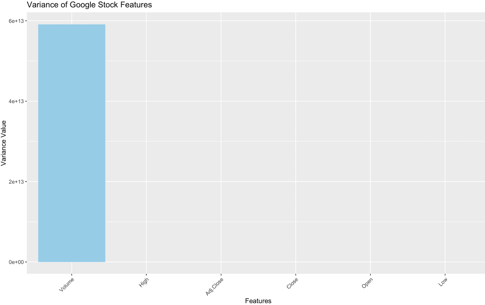
Visualizing the data distribution can provide insights into its spread and central tendencies.
Histograms and boxplots are commonly used for this purpose.
# Plotting histograms for each numerical column
google_data %>%
  select(-Date) %>%
  gather(key = "Features", value = "Value") %>%
  ggplot(aes(x = Value)) +
  geom_histogram(fill = "blue", color = "black", bins = 50) +
  facet_wrap(~ Features, scales = "free_x") +
  labs(title = "Distribution of Google Stock Features", x = "Value", y = "Frequency")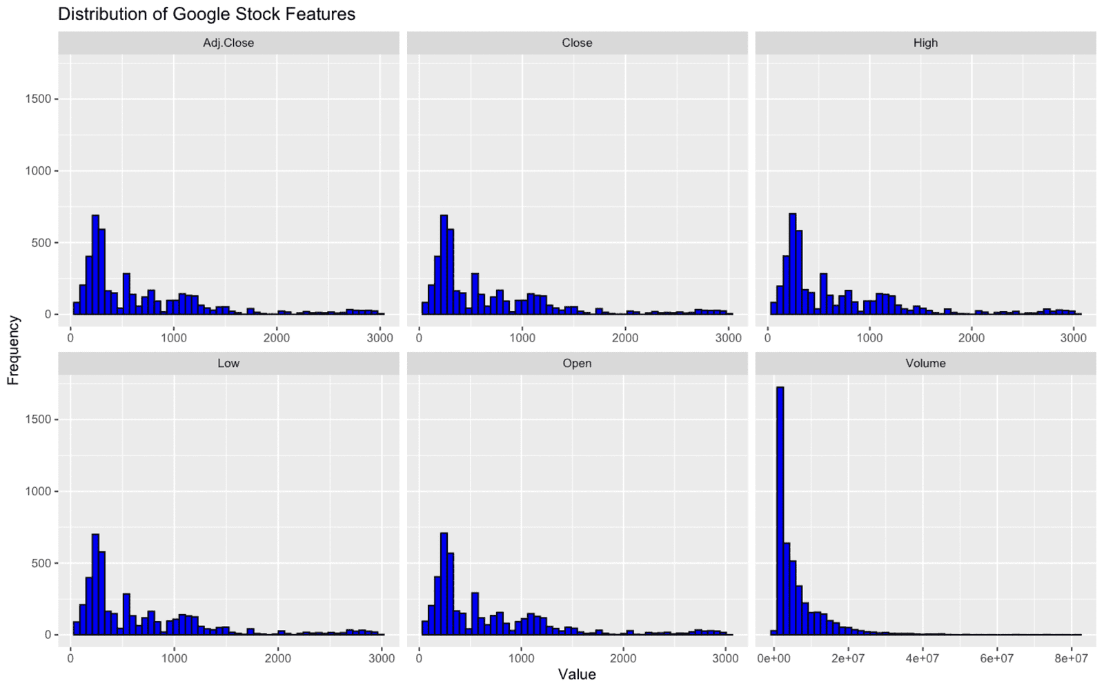
Sample Variance vs. Population Variance
The main difference between a sample and population variance relates to the variance calculation.
Population variance refers to the value of variance calculated from population data, and sample variance is the variance calculated from sample data.
The correction does not matter for large sample sizes. However, it does matter when the dataset has small sample sizes. When the variance is calculated from population data, n equals the number of elements.
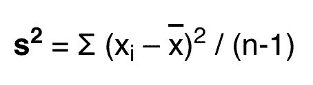
The formula of sample variance
The formula of population variance
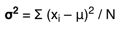
To calculate the population variance p (where the division is by n), you need to manually adjust the calculation:
mean((x - mean(x)) ^ 2)Here is a code example of this:
population_variance <- function(rv) {
 mean((rv - mean(rv)) ^ 2)
}

weights <- c(60, 55, 50, 65, 59)
population_variance(weights)
Output
[1] 25.36That’s it.

Krunal Lathiya is a seasoned Computer Science expert with over eight years in the tech industry. He boasts deep knowledge in Data Science and Machine Learning. Versed in Python, JavaScript, PHP, R, and Golang. Skilled in frameworks like Angular and React and platforms such as Node.js. His expertise spans both front-end and back-end development. His proficiency in the Python language stands as a testament to his versatility and commitment to the craft.