The summary() is a generic function that produces the summary statistics for various R objects, including vectors, matrices, data frames, and model objects.
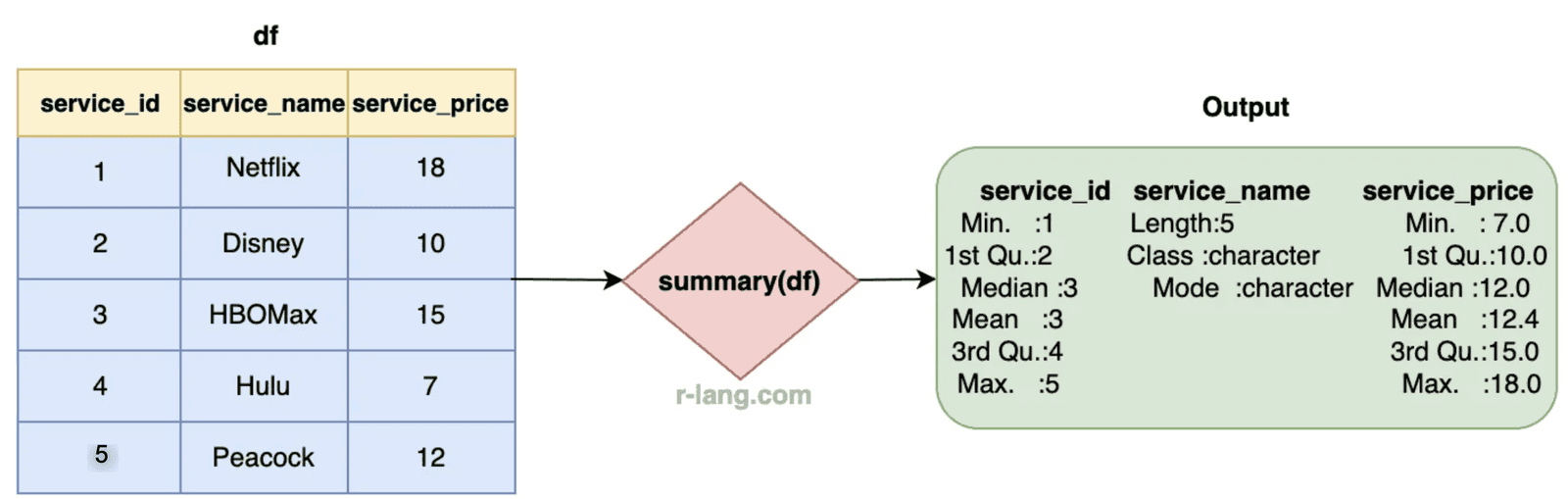
The above figure explains the summary for a data frame with three columns.
For different types of objects, the summary() function produces different types of summaries:
- If the input is numeric, it returns the minimum, 1st quartile, median, mean, 3rd quartile, and maximum.
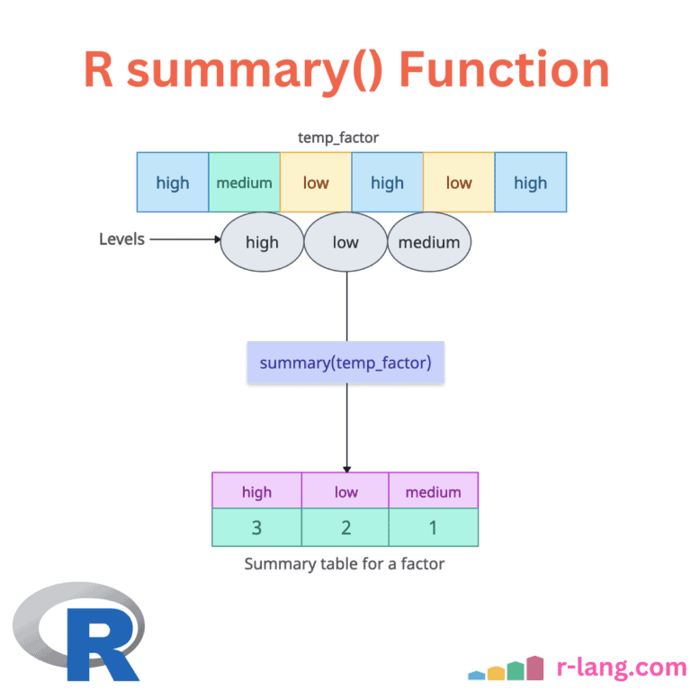
- If the input is categorical data such as factors, summary() returns a frequency table.
- For data frames, it applies the appropriate summary for each column.
- For model objects (like lm, glm), it produces a summary of the model fit, including coefficients, residuals, and significance tests.
Syntax
summary(object, …)Parameters
| Arguments | Description |
| object | It represents an R object, including a vector, a data frame, a matrix, a list, or a model object. |
Summary of data frame
To find the summary of a data frame, pass it to the summary() method, which returns the summary of each column appropriately (numeric/factor/character).
df <- data.frame(
  service_id = c(1:5),
  service_name = c("Netflix", "Disney+", "HBOMAX", "Hulu", "Peacock"),
  service_price = c(18, 10, 15, 7, 12),
  stringsAsFactors = FALSE
)

summary(df)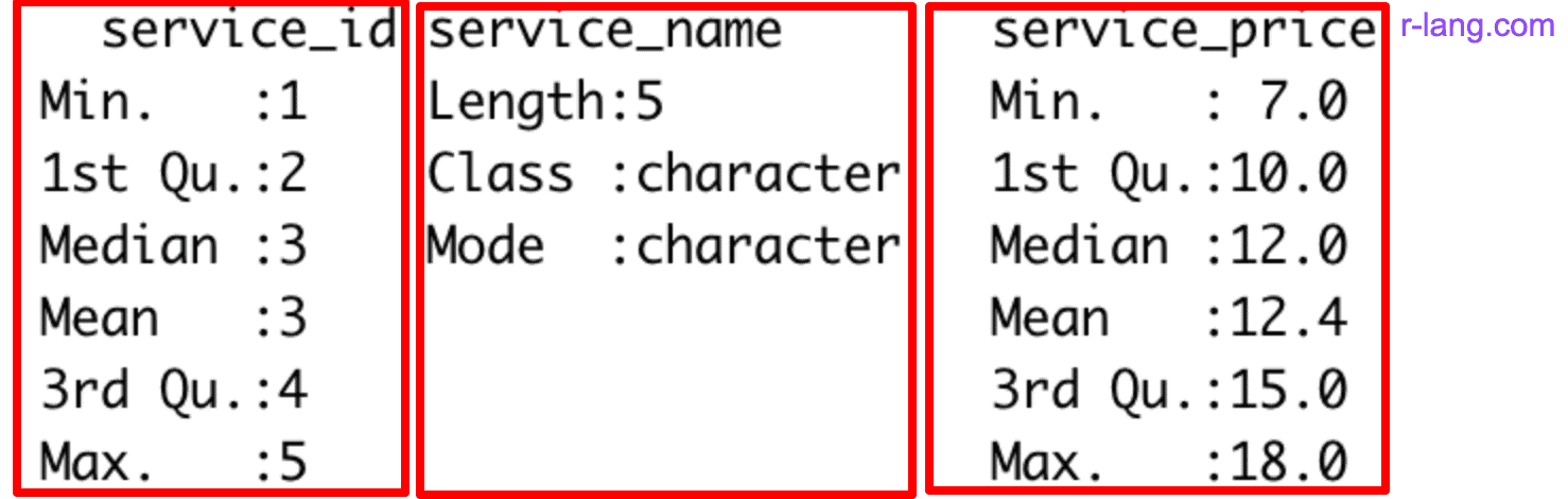
The above output shows the column-wise summary of the data frame.
The data frame contains three columns, and the summary is also provided for each column individually.
If you inspect carefully, the first column is numeric; in that case, the summary is different.
The second column is a character vector; its summary is different.
The third column is again a numeric vector, so its summary is the same as the first one except for different values.
Vector
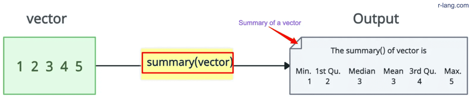
For a normal vector without containing NA values, it returns the minimum, Q1, median, mean, Q3, and maximum.
vec <- 1:5

summary(vec)

# Output:
#  Min.  1st Qu.   Median   Mean   3rd Qu.   Max.
#   1       2         3       3      4        5
Vector with NA values
If a vector contains missing values (NA), it also reports the count of NA values.
vec_with_na <- c(1, 2, NA, 4, 5, NA)

summary(vec_with_na)

# Output:

#  Min.   1st Qu.  Median   Mean   3rd Qu.  Max.   NA's
#  1.00     1.75     3.00   3.00    4.25    5.00    2
If you carefully analyze the above output, you will know that there are two NAs in the input vector.
Empty vector
summary(numeric(0))

# Output:

#  Min.  1st Qu.  Median  Mean  3rd Qu.  Max.
Factor / Categorical data
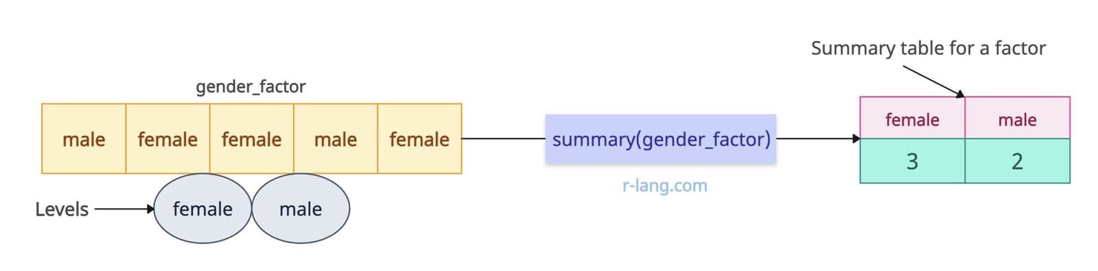
As we know, when you pass a factor to the summary() function, it returns a frequency table that contains the count of each element of the factor.
gender_factor <- factor(c("male", "female", "female", "male", "female"))

summary(gender_factor)

# Output:
# female   male
#   3       2
The above output shows that female appears 3 times and male appears 2 times in the factor.
List
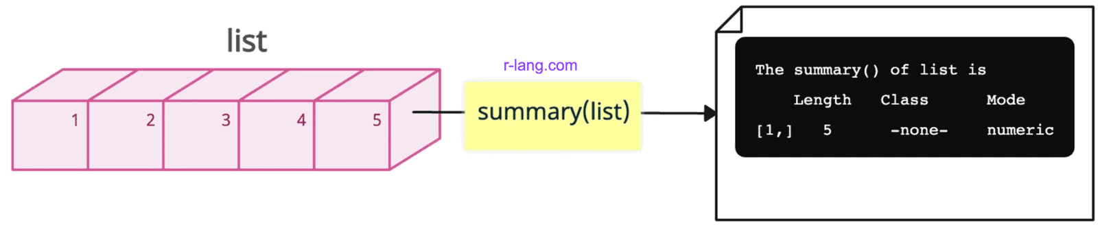
The summary of a list has Length, Class, and Mode attributes.
vec <- 1:5

list <- list(vec)

summary(list)

# Output:
#      Length  Class     Mode
# [1,]   5     -none-   numeric
Matrix
If the input matrix has two columns, the output will have two summaries. Again, it returns the summary column-wise.
rv <- c(11, 18, 19, 21)

mtrx <- matrix(rv, nrow = 2, ncol = 2)

summary(mtrx)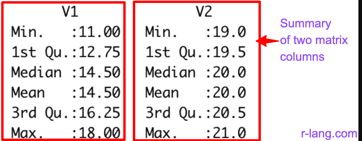
Summary of the linear regression model
Linear regression attempts to model the relationship between two variables by fitting a linear equation to observed data. One variable is considered an explanatory variable, and the other is a dependent variable.
A widespread application of the summary functions is the calculation of summary statistics of statistical models.
set.seed(93274)

l_x <- rnorm(1000)
l_y <- rnorm(1000) + l_x

mod <- lm(l_y ~ l_x)

summary(mod)
Output
Call:
lm(formula = l_y ~ l_x)

Residuals:
 Min 1Q Median 3Q Max
-3.7337 -0.6964 -0.0047 0.7333 3.3489

Coefficients:
 Estimate Std. Error t value Pr(>|t|)
(Intercept) -0.02159 0.03292 -0.656 0.512
l_x 1.00156 0.03262 30.707 <2e-16 ***
---
Signif. codes: 0 ‘***’ 0.001 ‘**’ 0.01 ‘*’ 0.05 ‘.’ 0.1 ‘ ’ 1

Residual standard error: 1.041 on 998 degrees of freedom
Multiple R-squared: 0.4858, Adjusted R-squared: 0.4853
F-statistic: 942.9 on 1 and 998 DF, p-value: < 2.2e-16
Summary of regression model: coefficients, p-values, R-squared, residuals, etc.
For more detailed or specific summaries, other functions like str(), table(), or specialized packages for statistical modeling might be necessary.

Krunal Lathiya is a seasoned Computer Science expert with over eight years in the tech industry. He boasts deep knowledge in Data Science and Machine Learning. Versed in Python, JavaScript, PHP, R, and Golang. Skilled in frameworks like Angular and React and platforms such as Node.js. His expertise spans both front-end and back-end development. His proficiency in the Python language stands as a testament to his versatility and commitment to the craft.