The pnorm() function in R calculates the cumulative density function (cdf) value of the normal distribution given a specific random variable q, the population mean μ, and the population standard deviation σ.

It returns the probability that a normally distributed random variable is less than or equal to a given value.
It provides the probability that a normally distributed random variable will be less than or equal to a specified value.
Syntax
pnorm(q, mean, sd, lower.tail = TRUE, log.p = FALSE)Parameters
| Argument | Description |
| q | It is a vector of quantiles. |
| mean | It is a vector of means. |
| sd | It is a vector of standard deviations. |
| lower.tail | It is logical; if TRUE (default), probabilities are otherwise. |
| log, log.p | It is a logical argument. |
Standard Normal Distribution (Default Parameters)
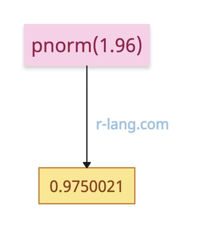
pnorm(1.96)

# Output: [1] 0.9750021
If we have a vector input, it calculates the pnorm element-wise.
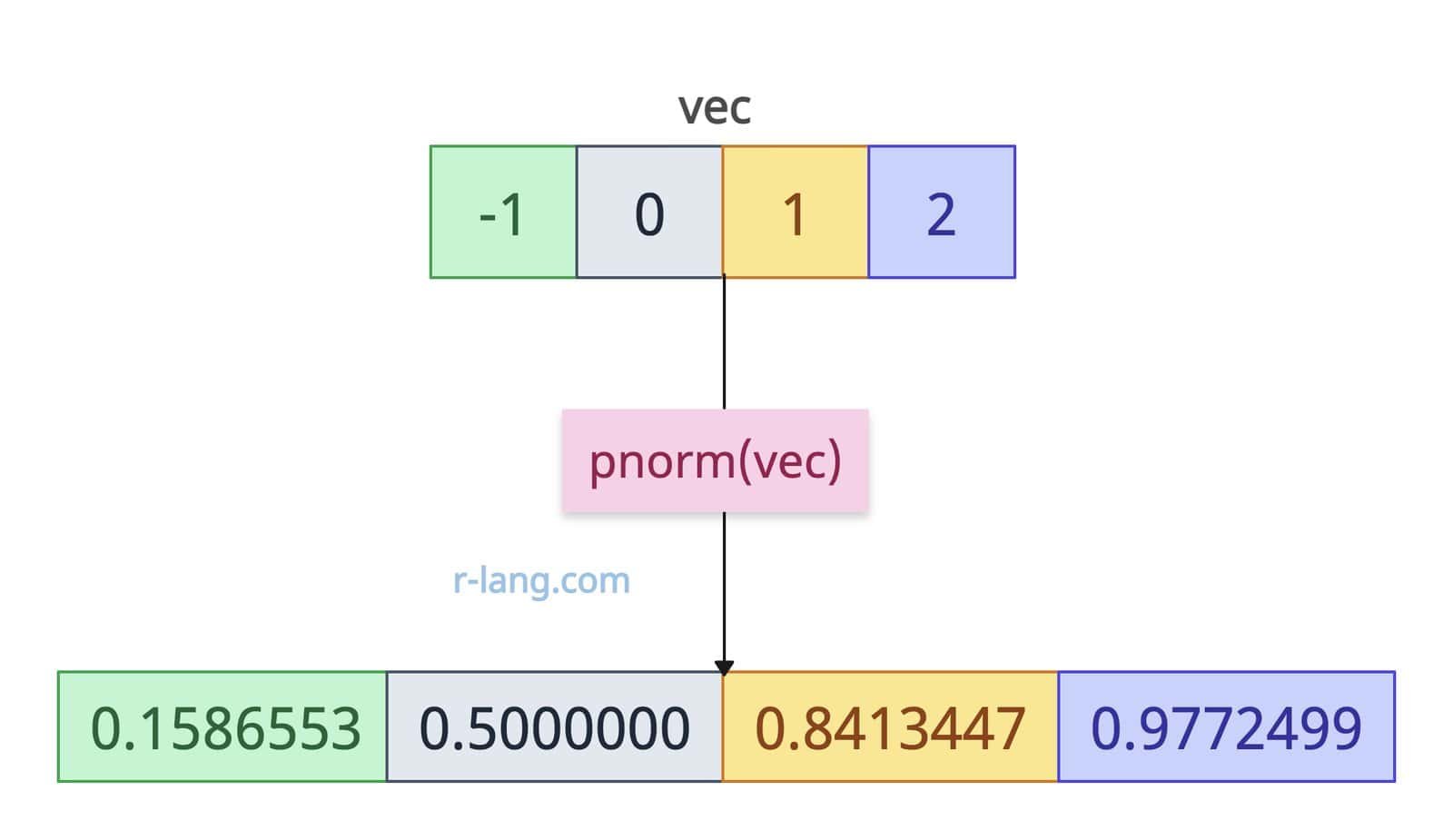
vec <- c(-1, 0, 1, 2)

pnorm(vec)

# Output: [1] 0.1586553 0.5000000 0.8413447 0.9772499
Extreme input values
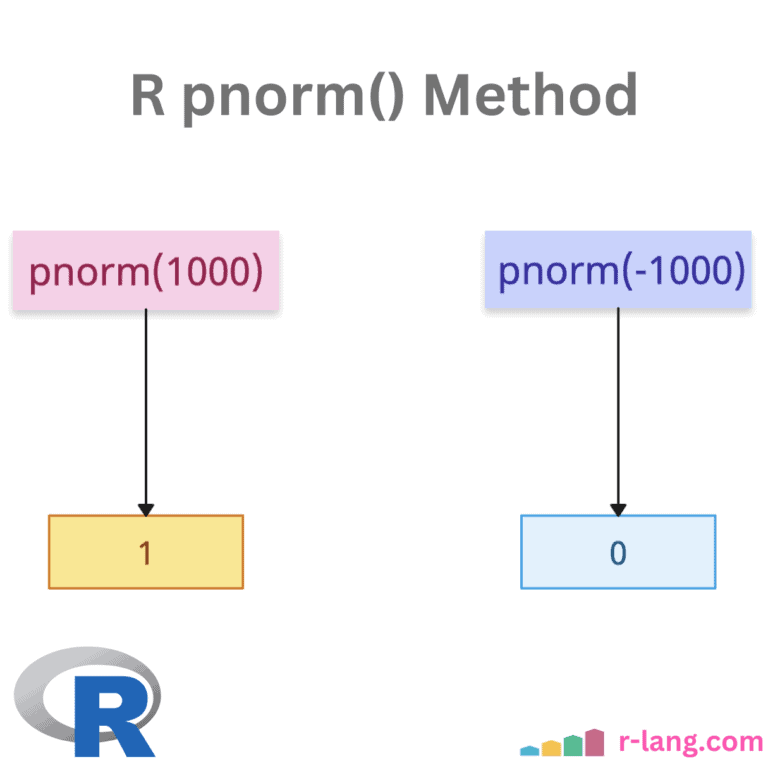
If the input value is 1000, it will output 1. But if you pass a negative value, what should be the output? Let’s find out.
pnorm(1000)
# Output: [1] 1 (Overflow-safe; returns 1 for extremely large q)

pnorm(-1000)
# Output: [1] 0
mean (optional, default = 0)
It is the mean (μ) of the normal distribution.
# Standard normal (mean = 0)
pnorm(1, mean = 0)
# Output: [1] 0.8413447

# Custom mean
pnorm(1, mean = 2)
# Output: [1] 0.1586553

pnorm(3, mean = 2)
# Output: [1] 0.8413447
sd (optional, default = 1)
It is the standard deviation (σ) of the normal distribution. It must be positive.
# Standard deviation = 1
pnorm(2, sd = 1)
# Output: [1] 0.9772499

# Standard deviation = 2
pnorm(2, sd = 2)
# Output: [1] 0.8413447

# Standard deviation = 0.5
pnorm(1, sd = 0.5)
# Output: [1] 0.9772499
Non-standard normal distribution
pnorm(78, mean = 74, sd = 2, lower.tail = FALSE)

# Output: [1] 0.02275013
Graphical representation
To visualize this function, we can plot the probability density function (PDF) of the normal distribution and shade the area to the right of x = 78, representing the right-tail probability.
We will use RStudio to plot the chart and the ggplot2 library. Install if you have not already!
# Load necessary libraries
library(ggplot2)

# Define parameters
mean_val <- 74
sd_val <- 2

# Create a sequence of x values
x <- seq(68, 80, by = 0.1)

# Calculate the PDF for the x values
y <- pnorm(x, mean = mean_val, sd = sd_val)

# Plot the PDF
p <- ggplot(data.frame(x = x, y = y), aes(x = x, y = y)) +
  geom_line() +
  geom_area(
  data = data.frame(x = x[x >= 78], y = y[x >= 78]),
  aes(x = x, y = y), fill = "skyblue"
 ) +
 geom_vline(aes(xintercept = 78), linetype = "dashed", color = "red") +
 labs(
   title = "Right-tail of Normal Distribution",
   x = "x",
   y = "Density"
 ) +
 theme_minimal()

# Display the plot
print(p)
Upper-Tail Probabilities
pnorm(1.96, lower.tail = FALSE)

# Output: [1] 0.0249979
Log Probability
log_p <- pnorm(2, log.p = TRUE)

exp(log_p)

# Output: [1] 0.9772499
Edge cases & errors
What if the inputs are 0, -inf, inf, or NA? What would the output? Let’s find out.
# Non-positive sd (error)
pnorm(0, sd = 0)
# Output: [1] 1

# Infinite values
pnorm(-Inf)
# Output: [1] 0.0

pnorm(Inf)
# Output: [1] 1.0

# Missing values
pnorm(NA)
# Output: [1] NA
That’s all!

Krunal Lathiya is a seasoned Computer Science expert with over eight years in the tech industry. He boasts deep knowledge in Data Science and Machine Learning. Versed in Python, JavaScript, PHP, R, and Golang. Skilled in frameworks like Angular and React and platforms such as Node.js. His expertise spans both front-end and back-end development. His proficiency in the Python language stands as a testament to his versatility and commitment to the craft.