Counting conditionally in the data frame means counting the number of rows that meet specific conditions defined by the user. It is the process of determining the number of rows based on certain conditions evaluated to TRUE.
You can count several rows conditionally in a data frame using base R functions, dplyr methods, or data.table functions.
Here is the demo dataset we are using:
fitness_data <- data.frame(
  User_ID = c("U001", "U002", "U003", "U004", "U005", "U006", "U007"),
  Activity_Type = c("Running", "Walking", "Cycling", "Running", "Walking", "Cycling", "Walking"),
  Steps_Taken = c(12000, 8000, 15000, 14500, 10500, 13200, 9800)
)

print(fitness_data)
Method 1: Using base R functions
The most basic way to count the number of rows conditionally is to use the sum() function with a logical vector.
Single condition
Let’s count rows based on a single condition:

fitness_data <- data.frame(
  User_ID = c("U001", "U002", "U003", "U004", "U005", "U006", "U007"),
  Activity_Type = c("Running", "Walking", "Cycling", "Running", "Walking", "Cycling", "Walking"),
  Steps_Taken = c(12000, 8000, 15000, 14500, 10500, 13200, 9800)
)

print(fitness_data)

sum(fitness_data$Activity_Type == "Walking")

# Output: [1] 3
The above figure and code indicate that only three rows have an Activity_Type of Walking. That’s it! It is conditional counting.
Multiple conditions
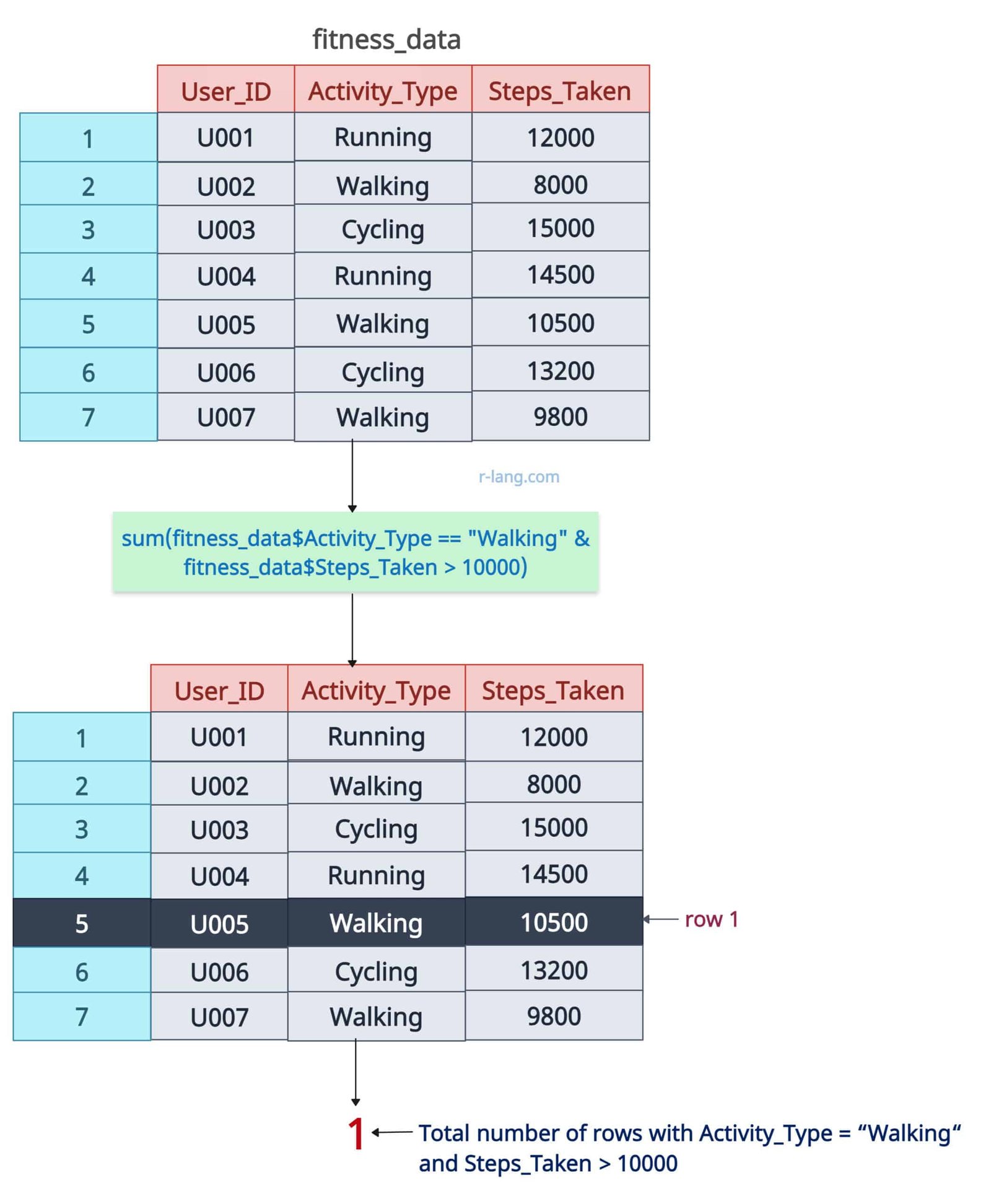
Count rows where Activity_Type is “Cycling” and Steps_Taken > 10,000. Here, two conditions are type cycling and steps greater than 10000.
fitness_data <- data.frame(
  User_ID = c("U001", "U002", "U003", "U004", "U005", "U006", "U007"),
  Activity_Type = c("Running", "Walking", "Cycling", "Running", "Walking", "Cycling", "Walking"),
  Steps_Taken = c(12000, 8000, 15000, 14500, 10500, 13200, 9800)
)

print(fitness_data)

# Multiple conditions

sum(fitness_data$Activity_Type == "Cycling" & fitness_data$Steps_Taken > 10000)
# Output: [1] 2
Subsetting with nrow()
We can also use the nrow() function to apply a condition to the data frame and return the count based on the condition.
Let’s count rows where Steps_Taken > 12000:

fitness_data <- data.frame(
  User_ID = c("U001", "U002", "U003", "U004", "U005", "U006", "U007"),
  Activity_Type = c("Running", "Walking", "Cycling", "Running", "Walking", "Cycling", "Walking"),
  Steps_Taken = c(12000, 8000, 15000, 14500, 10500, 13200, 9800)
)

print(fitness_data)

# Subsetting with nrow()

nrow(fitness_data[fitness_data$Steps_Taken > 12000, ])

# Output: [1] 3
Frequency tables
What is the purpose of the frequency table here? It returns the count of occurrences for each item shown in the table.
We need to pass the “categorical variable,” which is a column in the data frame, and it will return a table of values along with their respective counts.
fitness_data <- data.frame(
User_ID = c("U001", "U002", "U003", "U004", "U005", "U006", "U007"),
Activity_Type = c("Running", "Walking", "Cycling", "Running", "Walking", "Cycling", "Walking"),
Steps_Taken = c(12000, 8000, 15000, 14500, 10500, 13200, 9800)
)
print(fitness_data)
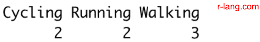
# Frequency Tables
table(fitness_data$Activity_Type)
Output
Method 2: Using dplyr
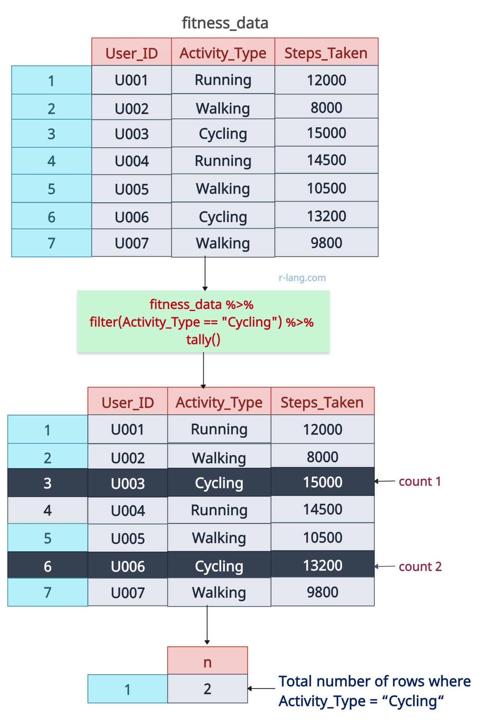
The dplyr::filter() function applies single or multiple conditions to a data frame that returns filtered rows, and then you can count those filtered rows using the tally() function.
Simple filtered count
Let’s count rows where Activity_Type is “Cycling”.
library(dplyr)

fitness_data <- data.frame(
  User_ID = c("U001", "U002", "U003", "U004", "U005", "U006", "U007"),
  Activity_Type = c("Running", "Walking", "Cycling", "Running", "Walking", "Cycling", "Walking"),
  Steps_Taken = c(12000, 8000, 15000, 14500, 10500, 13200, 9800)
)

print(fitness_data)


# Simple Filtering

fitness_data %>% filter(Activity_Type == "Cycling") %>% tally()
Output
Conditional grouped counts
The dplyr package provides the group_by() method to group data frames based on categorical columns. The summarize() function applies a condition and counts the number of rows based on that condition.
Let’s count users with Steps_Taken > 12000 per activity (group by Activity_Type).
library(dplyr)

fitness_data <- data.frame(
  User_ID = c("U001", "U002", "U003", "U004", "U005", "U006", "U007"),
  Activity_Type = c("Running", "Walking", "Cycling", "Running", "Walking", "Cycling", "Walking"),
  Steps_Taken = c(12000, 8000, 15000, 14500, 10500, 13200, 9800)
)

print(fitness_data)


# Conditional Grouped Counts
fitness_data %>%
  group_by(Activity_Type) %>%
  summarise(High_Step_Users = sum(Steps_Taken > 12000))
Output
 The dplyr approach is helpful when filtering, sorting, and grouping the data frame based on complex conditions. It supports all types of statistical operations.
Using the %>% operator, we can chain different functions to get the desired output.
Method 3: Using data.table functions
To use data.table, we first need to install and load the data.table package.
In the next step, we need to convert our input data frame into a data table using the setDT() function.
At last, we apply a condition where Activity_Type = “Running” and count only rows of that Activity.
library(data.table)


fitness_data <- data.frame(
  User_ID = c("U001", "U002", "U003", "U004", "U005", "U006", "U007"),
  Activity_Type = c("Running", "Walking", "Cycling", "Running", "Walking", "Cycling", "Walking"),
  Steps_Taken = c(12000, 8000, 15000, 14500, 10500, 13200, 9800)
)

print(fitness_data)

# Fast Filtering

setDT(fitness_data)

fitness_data[Activity_Type == "Running", .N]

# Output: 2
Grouped counting
Using the “by” argument, you can pass a categorical column through which you can group by your data.table and count the rows as per category.
Let’s count rows per Activity_Type:
library(data.table)


fitness_data <- data.frame(
  User_ID = c("U001", "U002", "U003", "U004", "U005", "U006", "U007"),
  Activity_Type = c("Running", "Walking", "Cycling", "Running", "Walking", "Cycling", "Walking"),
  Steps_Taken = c(12000, 8000, 15000, 14500, 10500, 13200, 9800)
)

print(fitness_data)


setDT(fitness_data)

# Counting the number of users for each activity type
fitness_data[, .N, by = Activity_Type]
Output
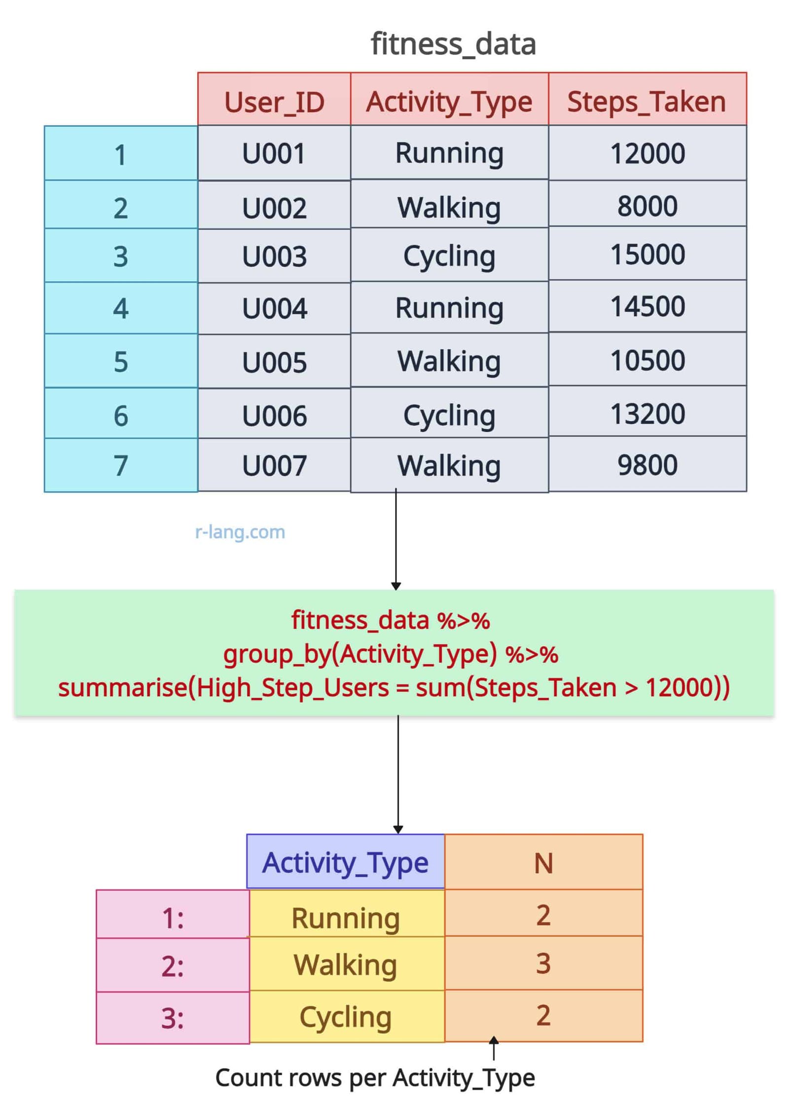
The data.table has 2 rows containing Activity_Type Running, 3 rows of Activity_Type Walking, and 2 rows of Activity_Type Cycling.
The data.table approach is highly recommended if your dataset is large.

Krunal Lathiya is a seasoned Computer Science expert with over eight years in the tech industry. He boasts deep knowledge in Data Science and Machine Learning. Versed in Python, JavaScript, PHP, R, and Golang. Skilled in frameworks like Angular and React and platforms such as Node.js. His expertise spans both front-end and back-end development. His proficiency in the Python language stands as a testament to his versatility and commitment to the craft.