The group_by() function from the dplyr package allows us to group data frames by one or more variables (columns), enabling subsequent operations to be performed on these groups.
For example, calculating the total sales for each category or counting the number of items in each category.
You cannot use the group_by() function alone because it returns nothing. It makes sense to use it when you want to use it with either aggregate functions or other dplyr functions, such as summarise(), mutate(), or filter(), within each group rather than the entire dataset.
Syntax
group_by(.data, .variables, .add = FALSE, .drop = group_by_drop_default(.df))
Parameters
| Argument | Value |
| .data | It is a data frame or tibble (an extended version of a data frame). |
| .variables | They are variables (columns) or computations to group by. Use commas to separate multiple variables |
| .add | If TRUE, it adds new groupings to existing ones (default FALSE replaces them). |
| .drop | If TRUE (default for Tibbles), it drops empty groups from factors with unused levels. |
Install and load the dplyr package
If you have not installed the dplyr package, you should install and load it using the library() function.
install.packages("dplyr")

library(dplyr)
Demo Data Frame
df_sales_data <- data.frame(
  Product = c("Apple", "Banana", "Milk", "Bread", "Butter", "Cheese"),
  Category = c("Fruit", "Fruit", "Dairy", "Bakery", "Dairy", "Dairy"),
  Price = c(1.2, 0.5, 2.5, 1.8, 2.0, 2.1),
  Quantity = c(5, 10, 2, 3, 12, 3),
  stringsAsFactors = FALSE
)

print(df_sales_data)
Basic grouping with summarise()
The summarise() is a dplyr function that helps calculate total sales or average price per Category. Total sales could be Price multiplied by Quantity.
library(dplyr)

df_sales_data <- data.frame(
  Product = c("Apple", "Banana", "Milk", "Bread", "Butter", "Cheese"),
  Category = c("Fruit", "Fruit", "Dairy", "Bakery", "Dairy", "Dairy"),
  Price = c(1.2, 0.5, 2.5, 1.8, 2.0, 2.1),
  Quantity = c(5, 10, 2, 3, 12, 3),
  stringsAsFactors = FALSE
)

print(df_sales_data)

# Calculating Total sales per Category using summarise()
df_sales_data %>%
  group_by(Category) %>%
  summarise(Total_Sales = sum(Price * Quantity))
Output

The above output figure shows that we got the 3×2 tibble in the output with a new column called “Total_Sales”, which is the computation of Price * Quantity for each Category.
Please note that we used only one variable (Category) for grouping.
Grouping by multiple variables
When working on a live project, you may encounter a scenario where you need to group the data frame by multiple variables. For example, you may want to find the total quantities sold per Product within each Category. Here, two variables are Product and Category.
library(dplyr)
df_sales_data <- data.frame(
Product = c("Apple", "Banana", "Milk", "Bread", "Butter", "Cheese"),
Category = c("Fruit", "Fruit", "Dairy", "Bakery", "Dairy", "Dairy"),
Price = c(1.2, 0.5, 2.5, 1.8, 2.0, 2.1),
Quantity = c(5, 10, 2, 3, 12, 3),
stringsAsFactors = FALSE
)
print(df_sales_data)
# Grouping by Multiple Variables - Total quantity per product in each category
df_sales_data %>%
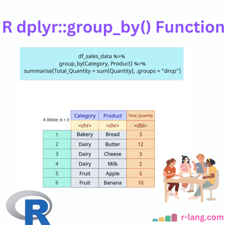
group_by(Category, Product) %>%
summarise(Total_Quantity = sum(Quantity), .groups = "drop")
Output

The above figure shows that we added a new variable called “Total_Quanity” based on Category and Product groupings. Total_Quantity is calculated using the sum() function.
Adding groupings with .add = TRUE
We can add already-grouped datasets using the .add = TRUE argument. For example, if your data set is already grouped by Category, you can add another group by Product using the .add = TRUE.
library(dplyr)

df_sales_data <- data.frame(
  Product = c("Apple", "Banana", "Milk", "Bread", "Butter", "Cheese"),
  Category = c("Fruit", "Fruit", "Dairy", "Bakery", "Dairy", "Dairy"),
  Price = c(1.2, 0.5, 2.5, 1.8, 2.0, 2.1),
  Quantity = c(5, 10, 2, 3, 12, 3),
 stringsAsFactors = FALSE
)

print(df_sales_data)

# Adding Groupings with .add = TRUE - Average price after adding product grouping
df_sales_data %>%
  group_by(Category) %>%
  group_by(Product, .add = TRUE) %>%
  summarise(Avg_Price = mean(Price), .groups = "drop")
Output

Retaining empty groups
By passing .drop = FALSE, we are telling R to retain an empty or non-existent group within the final tibble, including groups with zero rows (useful for factors with unused levels).
library(dplyr)

df_sales_data <- data.frame(
  Product = c("Apple", "Banana", "Milk", "Bread", "Butter", "Cheese"),
  Category = c("Fruit", "Fruit", "Dairy", "Bakery", "Dairy", "Dairy"),
  Price = c(1.2, 0.5, 2.5, 1.8, 2.0, 2.1),
  Quantity = c(5, 10, 2, 3, 12, 3),
  stringsAsFactors = FALSE
)

print(df_sales_data)

# Retaining Empty Groups - Include potential categories with no sales
df_sales_data %>%
  mutate(Category = factor(Category, levels = c("Fruit", "Dairy", "Bakery", "Biscuits"))) %>%
  group_by(Category, .drop = FALSE) %>%
  summarise(Total_Sales = sum(Price * Quantity))
Output
 The above figure shows that, due to “.drop = FALSE”, the output tibble includes the Biscuits with 0 to indicate the empty group in Total_Sales because the Category for that does not exist. If you pass .drop = TRUE, it won’t show an empty group in the final tibble.
Group-wise mutations
When you use functions after group_by(), like summarise(), each group is collapsed into a single row. In the case of mutate(), it returns the same number of rows but calculates within groups.
Let’s say I want to rank products by sales within each Category. To do that, you need to use the mutate() function.
library(dplyr)

df_sales_data <- data.frame(
  Product = c("Apple", "Banana", "Milk", "Bread", "Butter", "Cheese"),
  Category = c("Fruit", "Fruit", "Dairy", "Bakery", "Dairy", "Dairy"),
  Price = c(1.2, 0.5, 2.5, 1.8, 2.0, 2.1),
  Quantity = c(5, 10, 2, 3, 12, 3),
  stringsAsFactors = FALSE
)

print(df_sales_data)

# Group-Wise Mutations - Rank products by sales within categories
df_sales_data %>%
  group_by(Category) %>%
  mutate(
    Total_Sales = Price * Quantity,
    Sales_Rank = dense_rank(desc(Total_Sales))
  ) %>%
  select(Category, Product, Total_Sales, Sales_Rank)
Output

The above output figure shows that we calculated total sales for each Product and ranked them within their respective categories.
In the Fruit category, Apple has a total sales of 6, so it ranks 1. The same is true for Dairy, where Butter is ranked 1 because it has sales of 24, which is the highest.
Then, slightly fewer total sales for each category are assigned rank 2, and then rank 3 for the lowest sales.
Filtering groups
Group filtering involves first grouping the data based on a variable and then filtering that grouped data according to specific conditions.
For example, selecting the top 1 category by total sales, arranged by Category.
library(dplyr)

df_sales_data <- data.frame(
  Product = c("Apple", "Banana", "Milk", "Bread", "Butter", "Cheese"),
  Category = c("Fruit", "Fruit", "Dairy", "Bakery", "Dairy", "Dairy"),
  Price = c(1.2, 0.5, 2.5, 1.8, 2.0, 2.1),
  Quantity = c(5, 10, 2, 3, 12, 3),
  stringsAsFactors = FALSE
)

print(df_sales_data)

# Filtering Groups - Top one product per category by total sales
df_sales_data %>%
  group_by(Category) %>%
  mutate(Total_Sales = Price * Quantity) %>%
  slice_max(Total_Sales, n = 1) %>%
  arrange(Category)
Output

Keeping last row using group_by(), slice_tail(), and ungroup()
After grouping, you can use the slice_tail() function to keep the last row in each group using dplyr.
For example, if you are analyzing your transaction bill and want to check the most recent transaction by credit Category, you should look at the last row of that data set.
library(dplyr)

df_sales_data <- data.frame(
  Product = c("Apple", "Banana", "Milk", "Bread", "Butter", "Cheese"),
  Category = c("Fruit", "Fruit", "Dairy", "Bakery", "Dairy", "Dairy"),
  Price = c(1.2, 0.5, 2.5, 1.8, 2.0, 2.1),
  Quantity = c(5, 10, 2, 3, 12, 3),
  stringsAsFactors = FALSE
)

print(df_sales_data)

# Keeping the last row in each group
df_sales_data %>%
  group_by(Category) %>%
  slice_tail(n = 1) %>%
  ungroup()
Output

The above output image shows the last row from each category group.
The slice_tail(n = 1) method keeps the last row (n = 1) in each group by Category, and the ungroup() function removes the grouping structure after the operation.
That’s all!

Krunal Lathiya is a seasoned Computer Science expert with over eight years in the tech industry. He boasts deep knowledge in Data Science and Machine Learning. Versed in Python, JavaScript, PHP, R, and Golang. Skilled in frameworks like Angular and React and platforms such as Node.js. His expertise spans both front-end and back-end development. His proficiency in the Python language stands as a testament to his versatility and commitment to the craft.